Dirac equation

From Wikipedia, the free encyclopedia

Quantum physics

Introduction to...
Mathematical formulation of...

Fundamental concepts

Decoherence · Interference
Uncertainty · Exclusion
Transformation theory
Ehrenfest theorem · Measurement

Experiments

Double-slit experiment
Davisson-Germer experiment
Stern–Gerlach experiment
EPR paradox · Popper's experiment Schrödinger's cat

Equations

Schrödinger equation
Pauli equation
Klein-Gordon equation
Dirac equation

Advanced theories

Quantum field theory
Quantum electrodynamics
Quantum chromodynamics
Quantum gravity
Feynman diagram

Interpretations

Copenhagen · Quantum logic
Hidden variables · Transactional
Many-worlds · Ensemble
Consistent histories · Relational
Consciousness causes collapse
Orchestrated objective reduction

Scientists

Planck · Schrödinger
Heisenberg · Bohr · Pauli
Dirac · Bohm · Born
de Broglie · von Neumann
Einstein · Feynman
Everett · Others

This box: view • talk • edit

In physics, the Dirac equation is a relativistic quantum mechanical wave equation formulated by British physicist Paul Dirac in 1928 and provides a description of elementary spin-½ particles, such as electrons, consistent with both the principles of quantum mechanics and the theory of special relativity. The equation demands the existence of antiparticles and actually predated their experimental discovery, making the discovery of the positron, the antiparticle of the electron, one of the greatest triumphs of modern theoretical physics.

[edit] Details

The Dirac equation is

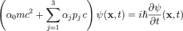
$\left(\alpha_0 mc^2 + \sum_{j = 1}^3 \alpha_j p_j \, c\right) \psi (\mathbf{x},t) = i \hbar \frac{\partial\psi}{\partial t}(\mathbf{x},t)$

where

m is the rest mass of the electron,

c is the speed of light,

p is the momentum operator,

$\hbar$ is the reduced Planck's constant,

x and t are the space and time coordinates respectively, and

ψ(x, t) is a four-component wavefunction. (The wavefunction has to be formulated as a four-component spinor, rather than a simple scalar, due to the demands of special relativity. The physical meanings of the components are discussed below.)

The α's are linear operators that act on the wavefunction. Their most fundamental property is that they must anticommute with each other. In other words,

$\alpha_i\alpha_j = -\alpha_j\alpha_i, \,$

where $i\ne j$ , and i and j range from zero to three. The simplest way to obtain such properties is with 4×4 matrices. There is no set of matrices of smaller dimension fulfilling the anticommutation requirements. The fact that four-dimensional matrices are necessary turns out to have physical significance.

[edit] Covariant form

Using Einstein summation notation, the covariant form of the Dirac equation may be written:

$i \hbar \gamma^\mu \partial_\mu \psi - m c \psi = 0 \,$

where

$\gamma^\mu\,$ is a four-vector of gamma matrices,

$\partial_\mu\,$ is the derivative with respect to component $μ$ ,

$c$ is the speed of light in vacuum,

$\hbar$ is the Reduced Planck's constant

m is the mass, and

$ψ$ is the field.

In addition, by defining

$\bar{\psi} = \psi^\dagger \gamma^0 \,$

we obtain the dirac equation for anti-particles:

$i \hbar \partial_\mu \bar{\psi} \gamma^\mu + m c \bar{\psi} = 0 \,$

[edit] History

Since the Dirac equation was originally invented to describe the electron, we will generally speak of "electrons" in this article. Actually, the equation also applies to quarks, which are also elementary spin-½ particles. A modified Dirac equation can be used to approximately describe protons and neutrons, which are not elementary particles (they are made up of quarks), but have a net spin of ½. Another modification of the Dirac equation, called the Majorana equation, is thought to describe neutrinos — also spin-½ particles.

The Dirac equation describes the probability amplitudes for a single electron. This is a single-particle theory; in other words, it does not account for the creation and destruction of the particles. It gives a good prediction of the magnetic moment of the electron and explains much of the fine structure observed in atomic spectral lines. It also explains the spin of the electron. Two of the four solutions of the equation correspond to the two spin states of the electron. The other two solutions make the peculiar prediction that there exist an infinite set of quantum states in which the electron possesses negative energy. This strange result led Dirac to predict, via a remarkable hypothesis known as "hole theory," the existence of particles behaving like positively-charged electrons. Dirac thought at first these particles might be protons. He was chagrined when the strict prediction of his equation (which actually specifies particles of the same mass as the electron) was verified by the discovery of the positron in 1932. When asked later why he hadn't actually boldly predicted the yet unfound positron with its correct mass, Dirac answered "Pure cowardice!" He shared the Nobel Prize anyway, in 1933.

Despite these successes, Dirac's theory is flawed by its neglect of the possibility of creating and destroying particles, one of the basic consequences of relativity. This difficulty is resolved by reformulating it as a quantum field theory. Adding a quantized electromagnetic field to this theory leads to the theory of quantum electrodynamics (QED). Moreover the equation cannot fully account for particles of negative energy but is restricted to positive energy particles.

A similar equation for spin 3/2 particles is called the Rarita-Schwinger equation.

[edit] Four spinor

Main article: Dirac spinor

The solutions to the Dirac equation can be separated into positive-energy solutions for particles and negative-energy solutions for anti-particles.

Both solutions are defined in terms of two-spinors, φ and χ, which have values depending on whether the particle is "spin up" or "spin down". Thus,

$\phi^1 = \chi^2 = \begin{bmatrix} 1 \\ 0 \end{bmatrix}, \quad \quad \phi^2 = \chi^1 = \begin{bmatrix} 0 \\ 1 \end{bmatrix} \,$

[edit] Positive energy solutions

The complete plane-wave solution for positive energy is

$\psi = u(p,s) e^{i p\cdot x} \,$

where u is a four-spinor of the form

$u(p,s) = \sqrt{E+m} \begin{bmatrix} \phi^s \\ \frac{\mathbf{\sigma \cdot p}}{E+m} \phi^s \end{bmatrix} \quad \mathrm{for} \ s = 1 \ \mathrm{or} \ 2 \,$ .

[edit] Negative energy solutions

For negative energy (anti-particles), the plane-wave solution is

$\psi = v(p,s) e^{i p\cdot x} \,$

where v is the four-spinor

$v(p,s) = \sqrt{E+m} \begin{bmatrix} \frac{\mathbf{\sigma \cdot p}}{E+m} \chi^s \\ \chi^s \end{bmatrix} \quad \mathrm{for} \ s = 1 \ \mathrm{or} \ 2 \,$ .

Note: the four-momentum for an anti-particle in this case is defined so they have negative energy and momentum

$p^\mu = (-E, -\mathbf{p}) \,$ .

[edit] Dirac matrices

Main article: Dirac matrices

A convenient (but not unique) choice of $α$ s is

$\gamma_0 = \begin{bmatrix} 1 & 0 & 0 & 0 \\ 0 & 1 & 0 & 0 \\ 0 & 0 & -1 & 0 \\ 0 & 0 & 0 & -1 \end{bmatrix}, \quad \gamma_1 = \begin{bmatrix} 0 & 0 & 0 & 1 \\ 0 & 0 & 1 & 0 \\ 0 & 1 & 0 & 0 \\ 1 & 0 & 0 & 0 \end{bmatrix},$

$\gamma_2 = \begin{bmatrix} 0 & 0 & 0 & -i \\ 0 & 0 & i & 0 \\ 0 & -i& 0 & 0 \\ i & 0 & 0 & 0 \end{bmatrix}, \quad \gamma_3 = \begin{bmatrix} 0 & 0 & 1 & 0 \\ 0 & 0 & 0 & -1 \\ 1 & 0 & 0 & 0 \\ 0 & -1 & 0 & 0 \end{bmatrix},$

known as Dirac matrices. All possible choices are related by similarity transformations because Dirac spinors are unique representation theoretically.

These matricies are often called gamma matrices, and they form a Clifford algebra whose defining property is

$\displaystyle\{ \gamma^\mu, \gamma^\nu \} = 2 \eta^{\mu \nu} I \,$

where

η is the Minkowski metric and

I is the Identity matrix.

[edit] Derivation of the Dirac equation

The Dirac equation is a relativistic extension of the Schrödinger equation, which describes the time-evolution of a quantum mechanical system:

$H \left| \psi (t) \right\rangle = i \hbar {d\over d t} \left| \psi (t) \right\rangle.$

For convenience, we will work in the position basis, in which the state of the system is represented by a wavefunction, ψ(x,t). In this basis, the Schrödinger equation becomes

$H \psi (\mathbf{x},t) = i \hbar \frac{\partial\psi}{\partial t} (\mathbf{x},t)$

where the Hamiltonian H now denotes an operator acting on wavefunctions rather than state vectors.

We have to specify the Hamiltonian so that it appropriately describes the total energy of the system in question. Let us consider a "free" electron isolated from all external force fields. For a non-relativistic model, we adopt a Hamiltonian analogous to the kinetic energy of classical mechanics (ignoring spin for the moment):

$H = \sum_{j=1}^3 \frac{p_j^2}{2m},$

where the p's are the momentum operators in each of the three spatial directions j=1,2,3. Each momentum operator acts on the wavefunction as a spatial derivative:

$p_j \psi(\mathbf{x},t) \ \stackrel{\mathrm{def}}{=}\ - i \hbar \, \frac{\partial\psi}{\partial x_j} (\mathbf{x},t)$

To describe a relativistic system, we have to find a different Hamiltonian. Assume that the momentum operators retain the above definition. According to Albert Einstein's famous mass-momentum-energy relationship, the total energy of a system is given by

$E = \sqrt{(mc^2)^2 + \sum_{j=1}^3 (p_jc)^2}.$

This prescribes something like

$\sqrt{(mc^2)^2 + \sum_{j=1}^3 (p_jc)^2} \; \psi = i \hbar \frac{d\psi}{d t}.$

This is not a satisfactory equation, for it does not treat time and space on an equal footing, one of the basic tenets of special relativity. The square of this equation leads to the Klein-Gordon equation. Dirac reasoned that, since the right side of the equation contains a first-order derivative in time, the left side should contain equally simple first-order derivatives in space (i.e., in the momentum operators). One way for this to happen is if the quantity in the square root is a perfect square. Suppose that you set

$E \cdot I = \alpha_0 mc^2 + c \sum_{i=1}^3 \alpha_i p_i.$

Here, I stands for the identity element. You'll gain the free Dirac equation:

$i\hbar \frac{d\psi}{dt} = \left[ c \sum_{i=1}^3 \alpha_i p_i + \alpha_0 mc^2 \right] \psi$

where the α's are constants to be determined thanks to the relativistic total energy.

$E^2 = (mc^2)^2 + \sum_{j=1}^3 (p_jc)^2 = \left( \alpha_0 mc^2 + \sum_{j=1}^3 \alpha_j p_j \, c \right)^2.$

Expanding the square and comparing coefficients on each side, we obtain the following conditions for the α's:

$\alpha_0^2 = I,$

$\alpha_i \alpha_0 + \alpha_0 \alpha_i = 0 \,, \quad i = 1,2,3,$

$\quad \alpha_i \alpha_j + \alpha_j \alpha_i = 2 \delta_{ij} \,,\quad i,j = 1, 2, 3.$

These last conditions may be written more concisely as

$\left\{\alpha_\mu , \alpha_\nu\right\} = 2\delta_{\mu \nu} \cdot I \,,\quad \mu,\nu = 0, 1, 2, 3$

where {...} is the anticommutator, defined as {A,B}≡AB+BA, and δ is the Kronecker delta, which has the value 1 if its two subscripts are equal and 0 otherwise. See Clifford algebra.

These conditions cannot be satisfied if the α's are ordinary numbers, but they can be satisfied if the α's are matrices. The matrices must be Hermitian, so that the Hamiltonian is Hermitian. The smallest matrices that work are 4×4 matrices, but there is more than one possible choice, or representation, of matrices. Although the choice of representation does not affect the properties of the Dirac equation, it does affect the physical meaning of the individual components of the wavefunction.

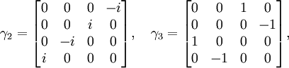
In the introduction, we presented the representation used by Dirac. This representation can be more compactly written as

$\alpha_0 = \begin{bmatrix} I & 0 \\ 0 & -I \end{bmatrix} \quad \alpha_j = \begin{bmatrix} 0 & \sigma_j \\ \sigma_j & 0 \end{bmatrix}$

where 0 and I are the 2×2 zero and identity matrices, respectively, and the σ_j's (j = 1, 2, 3) are the Pauli matrices.

The Hamiltonian in this equation,

$H = \,\alpha_0 mc^2 + \sum_{j = 1}^3 \alpha_j p_j \, c$

is called the Dirac Hamiltonian.

[edit] Quaternion representation

The Dirac equation can be written nicely in quaternion notation. We write it in terms of two quaternion fields representing the left-handed (Ψ) and right-handed (Φ) electrons:

$\partial_t\psi i + i \partial_x \psi+j \partial_y \psi + k\partial_z \psi= m_e \phi j,$

$\partial_t\phi i - i \partial_x \phi-j \partial_y \phi- k\partial_z \phi = m_e \psi j.$

It is important which side the unit quaternions are multiplied on for this to work. Notice that in the time and mass terms, the quaternions are multiplied on the right hand side. This representation of the Dirac equation is useful in such fields as computer simulation.

[edit] Nature of the wavefunction

Since the wavefunction ψ is acted on by the 4×4 Dirac matrices, it must be a four-component object. We will see, in the next section, that the wavefunction contains two sets of degrees of freedom, one associated with positive energies and the other with negative energies, with each set containing two degrees of freedom that describe the probability amplitudes for the spin to be pointing "up" or "down" along a specified direction.

We may explicitly write the wavefunction as a column matrix:

$\psi(\mathbf{x},t) \ \stackrel{\mathrm{def}}{=}\ \begin{bmatrix}\psi_1(\mathbf{x},t) \\ \psi_2(\mathbf{x},t) \\ \psi_3(\mathbf{x},t) \\ \psi_4(\mathbf{x},t) \end{bmatrix}.$

The dual wavefunction can be written as a row matrix:

$\psi^\dagger(\mathbf{x},t) \ \stackrel{\mathrm{def}}{=}\ \begin{bmatrix}\psi_1^*(\mathbf{x},t) & \psi_2^*(\mathbf{x},t) & \psi_3^*(\mathbf{x},t) & \psi_4^*(\mathbf{x},t) \end{bmatrix}$

where the * superscript denotes complex conjugation. By comparison, the dual of a scalar (one-component) wavefunction is just its complex conjugate.

As in ordinary single-particle quantum mechanics, the "absolute square" of the wavefunction gives the probability density of the particle at each position x and time t. In this case, the "absolute square" is the scalar product of the wavefunction with its dual:

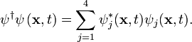
$\psi^\dagger \psi \, (\mathbf{x},t) = \sum_{j = 1}^4 \psi_j^*(\mathbf{x},t) \psi_j(\mathbf{x},t).$

The conservation of probability gives the normalization condition

$\int \psi^\dagger \psi \, (\mathbf{x},t) \; d^3x = 1.$

By applying Dirac's equation, we can examine the local flow of probability:

$\frac{\partial}{\partial t} \psi^\dagger \psi \, (\mathbf{x},t) = - \nabla \cdot \mathbf{J}.$

The probability current J is given by

$J_j = c \psi^\dagger \alpha_j \psi.$

Multiplying J by the electron charge e yields the electric current density j carried by the electron.

The values of the wavefunction components depend on the coordinate system. Dirac showed how ψ transforms under general changes of coordinate system, including rotations in three-dimensional space as well as Lorentz transformations between relativistic frames of reference. It turns out that ψ does not transform like a vector under rotations and is in fact a type of object known as a spinor.

[edit] Energy spectrum

It is instructive to find the energy eigenstates of the Dirac Hamiltonian. To do this, we must solve the time-independent Schrödinger equation,

$H \psi_0 (\mathbf{x}) = E \psi_0(\mathbf{x})$

where ψ₀ is the time-independent part of the energy eigenfunction

$\psi (\mathbf{x}, t) = \psi_0 (\mathbf{x}) e^{- i E t / \hbar}.$

Let us look for a plane-wave solution. For convenience, we align the z axis with the direction in which the particle is moving, so that

$\psi_0 = w e^{\frac{ipz}{\hbar}}$

where w is a constant four-component spinor and p is the momentum of the particle, as we can verify by applying the momentum operator to this wavefunction. In the Dirac representation, the equation for ψ₀ reduces to the eigenvalue equation:

$\begin{bmatrix} mc^2 & 0 & pc & 0 \\ 0 & mc^2 & 0 & -pc \\ pc & 0 & -mc^2 & 0 \\ 0 & -pc & 0 & -mc^2 \end{bmatrix} w = E w.$

For each value of p, there are two eigenspaces, both two-dimensional. One eigenspace contains positive eigenvalues, and the other negative eigenvalues, of the form

$E_\pm (p) = \pm \sqrt{(mc^2)^2 + (pc)^2}.$

The positive eigenspace is spanned by the eigenstates:

$\left\{ \begin{bmatrix}pc \\ 0 \\ \epsilon \\ 0 \end{bmatrix} \,,\, \begin{bmatrix}0 \\ pc \\ 0 \\ - \epsilon \end{bmatrix} \right\} \times \frac{1}{\sqrt{\epsilon^2+(pc)^2}}$

and the negative eigenspace by the eigenstates:

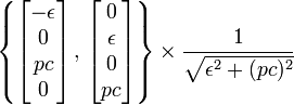
$\left\{ \begin{bmatrix}-\epsilon \\ 0 \\ pc \\ 0 \end{bmatrix} \,,\, \begin{bmatrix}0 \\ \epsilon \\ 0 \\ pc \end{bmatrix} \right\} \times \frac{1}{\sqrt{\epsilon^2+(pc)^2}}$

where

$\epsilon \ \stackrel{\mathrm{def}}{=}\ |E| - mc^2.$

The first spanning eigenstate in each eigenspace has spin pointing in the +z direction ("spin up"), and the second eigenstate has spin pointing in the −z direction ("spin down").

In the non-relativistic limit, the ε spinor component reduces to the kinetic energy of the particle, which is negligible compared to pc:

$\epsilon \sim \frac{p^2}{2m} \ll pc.$

In this limit, therefore, we can interpret the four wavefunction components as the respective amplitudes of (i) spin-up with positive energy, (ii) spin-down with positive energy, (iii) spin-up with negative energy, and (iv) spin-down with negative energy. This description is not accurate in the relativistic regime, where the non-zero spinor components have similar sizes.

[edit] Hole theory

The negative E solutions found in the preceding section are problematic, for it was assumed that the particle has a positive energy. Mathematically speaking, however, there seems to be no reason for us to reject the negative-energy solutions. Since they exist, we cannot simply ignore them, for once we include the interaction between the electron and the electromagnetic field, any electron placed in a positive-energy eigenstate would decay into negative-energy eigenstates of successively lower energy by emitting excess energy in the form of photons. Real electrons obviously do not behave in this way.

To cope with this problem, Dirac introduced the hypothesis, known as hole theory, that the vacuum is the many-body quantum state in which all the negative-energy electron eigenstates are occupied. This description of the vacuum as a "sea" of electrons is called the Dirac sea. Since the Pauli exclusion principle forbids electrons from occupying the same state, any additional electron would be forced to occupy a positive-energy eigenstate, and positive-energy electrons would be forbidden from decaying into negative-energy eigenstates.

Dirac further reasoned that if the negative-energy eigenstates are incompletely filled, each unoccupied eigenstate – called a hole – would behave like a positively charged particle. The hole possesses a positive energy, since energy is required to create a particle–hole pair from the vacuum. As noted above, Dirac initially thought that the hole might be the proton, but Hermann Weyl pointed out that the hole should behave as if it had the same mass as an electron, whereas the proton is over 1800 times heavier. The hole was eventually identified as the positron, experimentally discovered by Carl Anderson in 1932.

It is not entirely satisfactory to describe the "vacuum" using an infinite sea of negative-energy electrons. The infinitely negative contributions from the sea of negative-energy electrons has to be canceled by an infinite positive "bare" energy and the contribution to the charge density and current coming from the sea of negative-energy electrons is exactly canceled by an infinite positive "jellium" background so that the net electric charge density of the vacuum is zero. In quantum field theory, a Bogoliubov transformation on the creation and annihilation operators (turning an occupied negative-energy electron state into an unoccupied positive energy positron state and an unoccupied negative-energy electron state into an occupied positive energy positron state) allows us to bypass the Dirac sea formalism even though, formally, it is equivalent to it.

In certain applications of condensed matter physics, however, the underlying concepts of "hole theory" are valid. The sea of conduction electrons in an electrical conductor, called a Fermi sea, contains electrons with energies up to the chemical potential of the system. An unfilled state in the Fermi sea behaves like a positively-charged electron, though it is referred to as a "hole" rather than a "positron". The negative charge of the Fermi sea is balanced by the positively-charged ionic lattice of the material.

[edit] Electromagnetic interaction

So far, we have considered an electron that is not in contact with any external fields. Proceeding by analogy with the Hamiltonian of a charged particle in classical electrodynamics, we can modify the Dirac Hamiltonian to include the effect of an electromagnetic field. The revised Hamiltonian is (in SI units):

$H = \alpha_0 mc^2 + \sum_{j=1}^3 \alpha_j \left[p_j - e A_j(\mathbf{x}, t) \right] c + e \varphi(\mathbf{x}, t)$

where e is the electric charge of the electron (in this convention, e is negative), and A and φ are the electromagnetic vector and scalar potentials, respectively.

By setting φ = 0 and working in the non-relativistic limit, Dirac solved for the top two components in the positive-energy wavefunctions (which, as discussed earlier, are the dominant components in the non-relativistic limit), obtaining

$\left( \frac{1}{2m} \sum_j |p_j - e A_j(\mathbf{x}, t)|^2 - \frac{\hbar e}{2mc} \sum_j \sigma_j B_j(\mathbf{x}) \right) \begin{bmatrix}\psi_1 \\ \psi_2 \end{bmatrix}$
$= (E - mc^2) \begin{bmatrix}\psi_1 \\ \psi_2 \end{bmatrix}$

where B = $\nabla$ × A is the magnetic field acting on the particle. This is precisely the Pauli equation for a non-relativistic spin-½ particle, with magnetic moment $\hbar e/2mc$ (i.e., a spin g-factor of 2). The actual magnetic moment of the electron is larger than this, though only by about 0.12%. The shortfall is due to quantum fluctuations in the electromagnetic field, which have been neglected. See vertex function.

For several years after the discovery of the Dirac equation, most physicists believed that it also described the proton and the neutron, which are both spin-½ particles. However, beginning with the experiments of Stern and Frisch in 1933, the magnetic moments of these particles were found to disagree significantly with the predictions of the Dirac equation. The proton has a magnetic moment 2.79 times larger than predicted (with the proton mass inserted for m in the above formulas), i.e., a g-factor of 5.58. The neutron, which is electrically neutral, has a g-factor of −3.83. These "anomalous magnetic moments" were the first experimental indication that the proton and neutron are not elementary particles. They are in fact composed of smaller particles called quarks. Incidentally, quarks are spin-½ particles, which are exactly described by the Dirac equation !

[edit] Interaction Hamiltonian

It is noteworthy that the Hamiltonian can be written as the sum of two terms:

$H = H_{\mathrm{free}} + H_{\mathrm{int}} \,$

where H_free is the Dirac Hamiltonian for a free electron and H_int is the Hamiltonian of the electromagnetic interaction. The latter may be written as

$H_{\mathrm{int}} = e \varphi(\mathbf{x}, t) - ec \sum_{j=1}^3 \alpha_j A_j(\mathbf{x}, t).$

It has the expected value

$\langle H \rangle = \int \, \psi^\dagger H_{\mathrm{int}} \psi \, d^3x = \int \, \left(\rho \varphi - \sum_{i=1}^3 j_i A_i \right) \, d^3x$

where ρ is the electric charge density and j is the electric current density defined earlier. The integrand in the final expression is the interaction energy density. It is a relativistically covariant scalar quantity, as we can see by writing it in terms of the current-charge four-vector j = (ρc,j) and the potential four-vector A = (φ/c,A):

$\langle H \rangle = \int \, \left( \sum_{\mu,\nu = 0}^3 \eta^{\mu\nu} j_\mu A_\nu \right) \; d^3r$

where η is the metric of flat spacetime:

$η 00 = 1,$

$\eta^{ii} \;= -1 \quad\, \forall \, i=1,2,3,$

$\eta^{\mu\nu} = 0 \qquad \forall \, \mu \ne \nu.$

[edit] Lagrangian

The classical Lagrangian density of a spin 1/2 fermion with a mass "m" and parity invariance is given by

$\mathcal{L} = \frac{i}{2}\overline{\psi} \gamma^\mu \partial_\mu \psi -\frac{i}{2}\left(\partial_\mu \overline{\psi}\right) \gamma^\mu \psi -m\overline{\psi}\psi \,$

where

$\overline{\psi} = \psi^\dagger \gamma^0. \,$

To obtain an equation of motion, one can plug this lagrangian into the Euler-Lagrange equation:

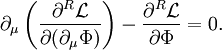
$\partial_\mu \left( \frac{\partial^{R} \mathcal{L}}{\partial ( \partial_\mu \Phi)} \right) - \frac{\partial^{R} \mathcal{L}}{\partial \Phi} = 0. \,$

where the upperscript "R" stands for the right derivative, and the $Φ$ is an arbitrary classical field (possibly fermionic).

Evaluating the two terms separately:

$\frac{\partial^{R} \mathcal{L}}{\partial (\partial_\mu \psi) } = \frac{i}{2}\overline{\psi} \gamma^\mu \,$

$\frac{\partial^{R} \mathcal{L}}{\partial \psi} = -\frac{i}{2}\left(\partial_{\mu}\overline{\psi}\right)\gamma^{\mu}- m \overline{\psi} \,$

Plugging those back into the Euler-Lagrange equation results in

$i \left(\partial_\mu \overline{\psi}\right) \gamma^\mu + m \overline{\psi} = 0 \,$

which is the Dirac equation for the conjugate spinor $\overline{\psi}$ .

We redo the calculations for the Dirac spinor $ψ$ , i.e. we evaluate

$\frac{\partial^{R} \mathcal{L}}{\partial (\partial_\mu \overline{\psi}) } = \frac{i}{2}\gamma^\mu \psi \,$

$\frac{\partial^{R} \mathcal{L}}{\partial \overline{\psi}} = -\frac{i}{2}\gamma^{\mu}\partial_{\mu}\psi + m \psi \,$

and get the Dirac equation

$i\gamma^{\mu}\partial_{\mu}\psi-m\psi =0$ .

[edit] Relativistically covariant notation

Let us return to the Dirac equation for the free electron. It is often useful to write the equation in a relativistically covariant form, in which the derivatives with time and space are treated on the same footing.

To do this, first recall that the momentum operator p acts like a spatial derivative:

$\mathbf{p} \psi(\mathbf{x},t) = - i \hbar \nabla \psi(\mathbf{x},t).$

Multiplying each side of the Dirac equation by α₀ (recalling that α₀²=I) and plugging in the above definition of p, we obtain

$\left[ i\hbar c \left(\alpha_0 \frac{\partial}{c \partial t} + \sum_{j=1}^3 \alpha_0 \alpha_j \frac{\partial}{\partial x_j} \right) - mc^2 \right] \psi = 0.$

Now, define four gamma matrices:

$\gamma^0 \ \stackrel{\mathrm{def}}{=}\ \alpha_0 \,,\quad \gamma^j \ \stackrel{\mathrm{def}}{=}\ \alpha_0 \alpha_j.$

These matrices possess the property that

$\left\{\gamma^\mu , \gamma^\nu \right\} = 2\eta^{\mu\nu} \cdot I\,,\quad \mu,\nu = 0, 1, 2, 3$

where η once again stands for the metric of flat spacetime. These relations define a Clifford algebra called the Dirac algebra.

The Dirac equation may now be written, using the position-time four-vector x = (ct,x), as

$\left(i\hbar c \, \sum_{\mu=0}^3 \; \gamma^\mu \, \partial_\mu - mc^2 \right) \psi = 0.$

With this notation, the Dirac equation can be generated by extremising the action

$\mathcal{S} = \int \bar\psi(i \hbar c \, \sum_\mu \gamma^\mu \partial_\mu - mc^2)\psi \, d^4 x$

where

$\bar\psi \ \stackrel{\mathrm{def}}{=}\ \psi^\dagger \gamma_0$

is called the Dirac adjoint of ψ. This is the basis for the use of the Dirac equation in quantum field theory.

A notation called the "Feynman slash" is sometimes used. Writing

$a\!\!\!/ \; \overset{\underset{\mathrm{def}}{}}{=} \sum_\mu \gamma^\mu a_\mu$

the Dirac equation becomes

$(i \hbar c \, \partial\!\!\!/ - mc^2) \psi = 0$

and the expression for the action becomes

$\mathcal{S} = \int \bar\psi(i \hbar c \, \partial \!\!\!/ - mc^2)\psi \, d^4 x.$

In this notation electromagnetic interaction can be added simply by promoting the partial derivative to gauge covariant derivative:

$\partial_\mu \rightarrow D_\mu = \partial_\mu - i e A_\mu.$

[edit] Dirac bilinears

There are five different (neutral) Dirac bilinear terms not involving any derivatives:

(S)calar: $\bar{\psi} \psi$ (scalar, P-even)
(P)seudoscalar: $\bar{\psi} \gamma^5 \psi$ (scalar, P-odd)
(V)ector: $\bar{\psi} \gamma^\mu \psi$ (vector, P-even)
(A)xial: $\bar{\psi} \gamma^\mu \gamma^5 \psi$ (vector, P-odd)
(T)ensor: $\bar{\psi} \sigma^{\mu\nu} \psi$ (antisymmetric tensor, P-even),

where $\sigma^{\mu\nu}=\frac{i}{2} \left[\gamma^{\mu},\gamma^{\nu}\right]_{-}$ and $\gamma^{5}=\gamma_{5}=\frac{i}{4!}\epsilon_{\mu\nu\rho\lambda}\gamma^{\mu}\gamma^{\nu}\gamma^{\rho}\gamma^{\lambda}=i\gamma^{0}\gamma^{1}\gamma^{2}\gamma^{3}$ .

A Dirac mass term is an S coupling. A Yukawa coupling may be S or P. The electromagnetic coupling is V. The weak interactions are V-A.

[edit] See also

[edit] References

[edit] Selected papers

P.A.M. Dirac "The Quantum Theory of the Electron", Proc. R. Soc. A117) link to the volume of the Proceedings of the Royal Society of London containing the article at page 610
P.A.M. Dirac "A Theory of Electrons and Protons", Proc. R. Soc. A126) link to the volume of the Proceedings of the Royal Society of London containing the article at page 360
C.D. Anderson, Phys. Rev. 43,)
R. Frisch and O. Stern, Z. Phys. 85 4 (1933)

[edit] Textbooks

Halzen, Francis; Martin, Alan (1984). Quarks & Leptons: An Introductory Course in Modern Particle Physics. John Wiley & Sons. ISBN.
Dirac, P.A.M., Principles of Quantum Mechanics, 4th edition (Clarendon, 1982)
Shankar, R., Principles of Quantum Mechanics, 2nd edition (Plenum, 1994)
Bjorken, J D & Drell, S, Relativistic Quantum mechanics
Thaller, B., The Dirac Equation, Texts and Monographs in Physics (Springer, 1992)
Schiff, L.I., Quantum Mechanics, 3rd edition (McGraw-Hill, 1955)

Retrieved from "http://en.wikipedia.org/wiki/Dirac_equation"

Categories: Fundamental physics concepts | Quantum field theory | Spinors | Partial differential equations | Fermions

Dirac equation

From Wikipedia, the free encyclopedia

Contents

[edit] Details

[edit] Covariant form

[edit] History

[edit] Four spinor

[edit] Positive energy solutions

[edit] Negative energy solutions

[edit] Dirac matrices

[edit] Derivation of the Dirac equation

[edit] Quaternion representation

[edit] Nature of the wavefunction

[edit] Energy spectrum

[edit] Hole theory

[edit] Electromagnetic interaction

[edit] Interaction Hamiltonian

[edit] Lagrangian

[edit] Relativistically covariant notation

[edit] Dirac bilinears

[edit] See also

[edit] References

[edit] Selected papers

[edit] Textbooks

Views

Personal tools

Navigation

interaction

Search

Toolbox

In other languages

From Wikipedia, the free encyclopedia

Contents

[edit] Details

[edit] Covariant form

[edit] History

[edit] Four spinor

[edit] Positive energy solutions

[edit] Negative energy solutions

[edit] Dirac matrices

[edit] Derivation of the Dirac equation

[edit] Quaternion representation

[edit] Nature of the wavefunction

[edit] Energy spectrum

[edit] Hole theory

[edit] Electromagnetic interaction

[edit] Interaction Hamiltonian

[edit] Lagrangian

[edit] Relativistically covariant notation

[edit] Dirac bilinears

[edit] See also

[edit] References

[edit] Selected papers

[edit] Textbooks

Views

Personal tools

if (window.isMSIE55) fixalpha(); Navigation

interaction

Search

Toolbox

In other languages

Navigation